Highly scattering materials like milk or skin can’t be precisely modeled by BRDF only, because light would scatter multiple times before exiting the material at different locations. Bidirectional surface scattering distribution function (BSSRDF) is used to describe radiance transfer across the surface boundary with diffusion profile for multiple scattering events.
To solve subsurface light transport efficiently, there are several approaches to model and evaluate the diffusion profile. Recently, Burley [5] has proposed an artist-friendly diffusion profile with only two exponential functions and the most attracting thing is that it’s not only intuitive for artists to use but also faster to evaluate. It’s a great exercise to try it out for fun in Arnold.
BSSRDF & Diffusion Profile
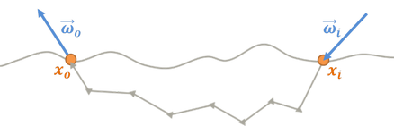
BSSRDF is a function relates outgoing radiance to the incident flux at different points:
$$S(x_i,\vec{\omega_i};x_o,\vec{\omega_o})=\frac{dL_o(x_o,\vec{\omega_o})}{d\phi_i(x_i,\vec{\omega_i})}$$
For efficiency, \(S\) can be decomposed into single-scattering and multiple-scattering terms. The multiple scatter term \(S_d\) is too complex to solve directly, the common strategy is to use a diffusion profile to approximate the distribution of outgoing radiance. With the diffusion approximation to the radiative transport equation (RTE), \(S_d\) is represented by a product of two Fresnel refraction terms and a diffusion profile in BSSRDF:
$$S_d(x_i,\vec{\omega_i};x_o,\vec{\omega_o})=\frac{1}{\pi}F_t(\eta,\vec{\omega_i})R_d(\vert x_i-x_o\vert)F_t(\eta,\vec{\omega_o})$$
and the subsurface light transport is formulated as:
$$L_o(x_o,\vec{\omega_o}) = \int_A{ \int_\Omega{ S(x_i,\vec{\omega_i};x_o,\vec{\omega_o}) L_i(x_i,\vec{\omega_i}) (n\cdot\vec{\omega_i}) d\omega_i } dA(x_i) }$$
There are many technical terms among the academic papers, such as fluence, mean free path, etc. I found the best introductory reading materials to understand the relevant details of sub-surface scattering approximation are:
- A Practical Model for Subsurface Light Transport. Jensen et al. 2001.
- Towards Realistic Image Synthesis of Scattering Materials. Donner. 2006.
- Classical and Improved Diffusion Theory for Subsurface Scattering. Ralf Habel et al. 2013.
About the diffusion profiles, there are several profiles such as diploe, multipole, quantized diffusion and directional dipole. The presentation slides of directional profile [J. R. Frisvad et al. 2014] has great illustrations for the integration scheme of each diffusion profile.
BSSRDF Importance Sampling Framework in Arnold
To solve the subsurface light transport, two primary approaches are used in graphics community. One is a multi-pass technique, which uses point cloud over the surface to store the diffuse irradiance at each point in pre-processing stage, then utilize that irradiance cache to solve the light transport equation in second phase.
The other is to perform importance sampling of the diffusion profile directly. Without the needs of point cloud generation, this approach fits well in any path-tracer with probe tracing API. The state-of-the-art sampling method proposed by King et al. [4] can be summarized to following steps:
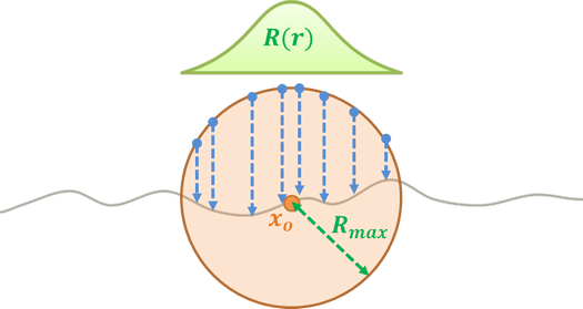
- Sample a point on disk with PDF in proportion to the diffusion profile \(R(r)\).
- Randomly select probe orientation with local basis U, V, N at \(x_o\).
- Compute probe origin and direction from the selected orientation.
- Trace probe rays to shade all hit points within a range of max radius.
- Combine sample results with MIS (Multiple Importance Sampling): $$w_i = \frac{R_d(|x_o-x_i|)}{\sum_j{c_j\ pdf_{disk}(r_j) |\vec{n_o}\cdot\vec{n_i}|}}\kern{2em}$$ where \(c_j\) is the sample weight of probe axis selection (N:0.5, U:0.25, V:0.25), and \(r_j\) is the projected radius on UV, NV, NU plane.
Arnold SDK only provides APIs for Gaussian and cubic profile currently, for other profiles, we have to implement the sampling routine from scratch. The implementation details would be discussed in later section. Now, let’s see how to sample the radius \(r\) from the normalized diffusion profile \(R(r)\).
Importance Sampling of Normalized Diffusion
Normalized diffusion profile [5][6] is formulated by two exponential functions:
$$R(r)=\frac{e^{\frac{-r}{d}} + e^{\frac{-r}{3d}}}{8\pi\ d\ r}$$
and the beauty of this model is that when evaluating the diffusion contribution with any positive value of \(d\), the integration over the disk is always one:
$$\int_0^\infty{\int_0^{2\pi}{R(r)\ r\ d\phi}\ dr}=\int_0^\infty{R(r)\ 2\pi r\ dr}=1$$
(The parameter \(d\) can be interpreted as the scattering distance for artistic control. For its relationship to other physical quantities like surface albedo and mean free path, please refer to [6])
Although \(R(r)\) is surprising simple, but its CDF is not analytically invertible. Therefore, I try to randomly select one exponential and generate sample \(r\) from it, then use MIS to combine the sample weights. Besides, in order to make probe tracing faster and to reduce the variance (noise), it’s better to restrict the integration domain within a user defined max radius \(R_{max}\).
Lobe selection
There are two exponential functions and three distance values \(d\) for R, G, B. In other words, there are six lobes to sample. Before sampling the radius \(r\) on disk, we need to select a lobe in two steps:
- Choose the value of \(d\) from R, G, B uniformly.
- Since every positive \(d\) would always get one for the integral of \(R(r)\).
- Given \(d\), use the ratio of integration within \(R_{max}\) to select the exponential function:
Sample \(r\) from a lobe
Suppose the PDF of the first exponential is \(p_1(r) \propto \frac{e^{-r/d}}{8\pi\ d\ r}\), and it’s normalized in range \([0, R_{max}]\). To get \(p_1 (r )\), let \(p_1 (r ) = c \times \frac{e^{-r/d}}{8\pi\ d\ r}, c \in \R \) and set its integral equal to one for solving the specific constant \(c\) makes \(p_1( r )\) normalized:
After we get \(p_1\), we could perform the integral in \([0, r]\) to get its CDF \(P_1(r )\):
Then we could get the inverse function \(P_1^{-1}(\xi)\) which maps \(\xi \in [0, 1]\) to distance r in \([0, R_{max}]\):
$$r = \log(1-\xi(1-e^{\frac{-R_{max}}{d}})) \times -d$$
Likewise, we can get the following formulas for the second exponential:
Implementation Details
Retrieve Correct Hit States from AiTraceProbe
During surface shading computation, the shading context of sg is AI_CONTEXT_SURFACE, and I found AiTraceProbe would always return false when the probe ray hits an identical triangle to the one stored in previous sg. To resolve this issue, at first I try to switch its shading context to AI_CONTEXT_DISPLACEMENT before each AiTraceProbe, then I found we could simply change sg->fi (the id of hit primitive) to UI_MAX to make it work properly.
In addition, about direct lighting evaluation, it would crash at AiLightsPrepare if we pass the returned AtShaderGlobals from AiTraceProbe directly. Thus we have to copy related information like P, Nf, Ng from in-scatter point to original sg before evaluating the light loop.
Stackless Shading For Multiple Probe Hits
To shade thin geometry correctly, we need to shade multiple hits along the probing direction. Although we could use shader message passing API to carry the shading samples along the ray, but AiTrace would increase the number of call stacks and slow down the rendering. Therefore, I use AiTraceProbe to retrieve the hit information and integrate direct/indirect illumination at each hit point.
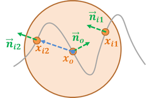
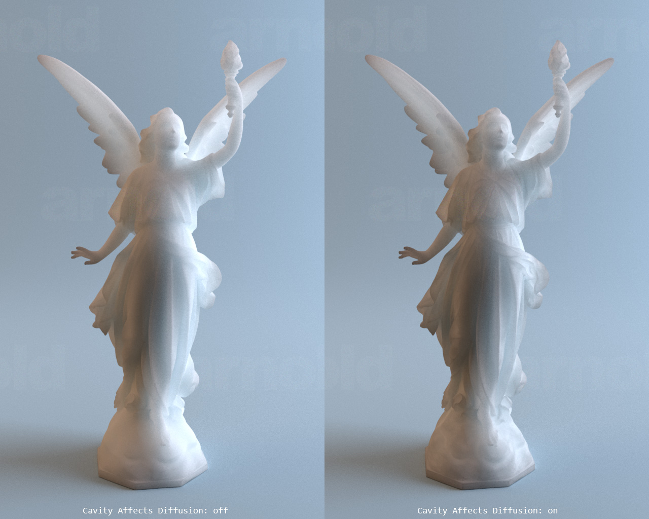
Reduce Incoming Radiance From Opposite Faces
Sometimes the energy from opposite faces would make the result too bright and need further reduction. For the consideration of surface cavity, I currently use \(\cos{\theta/2}\) to fade out the incoming radiance. Where the \(\theta\) is determined differently for front-facing (\(x_{i1}\)) and back-facing (\(x_{i2}\)) cases:
The source code could be found here.
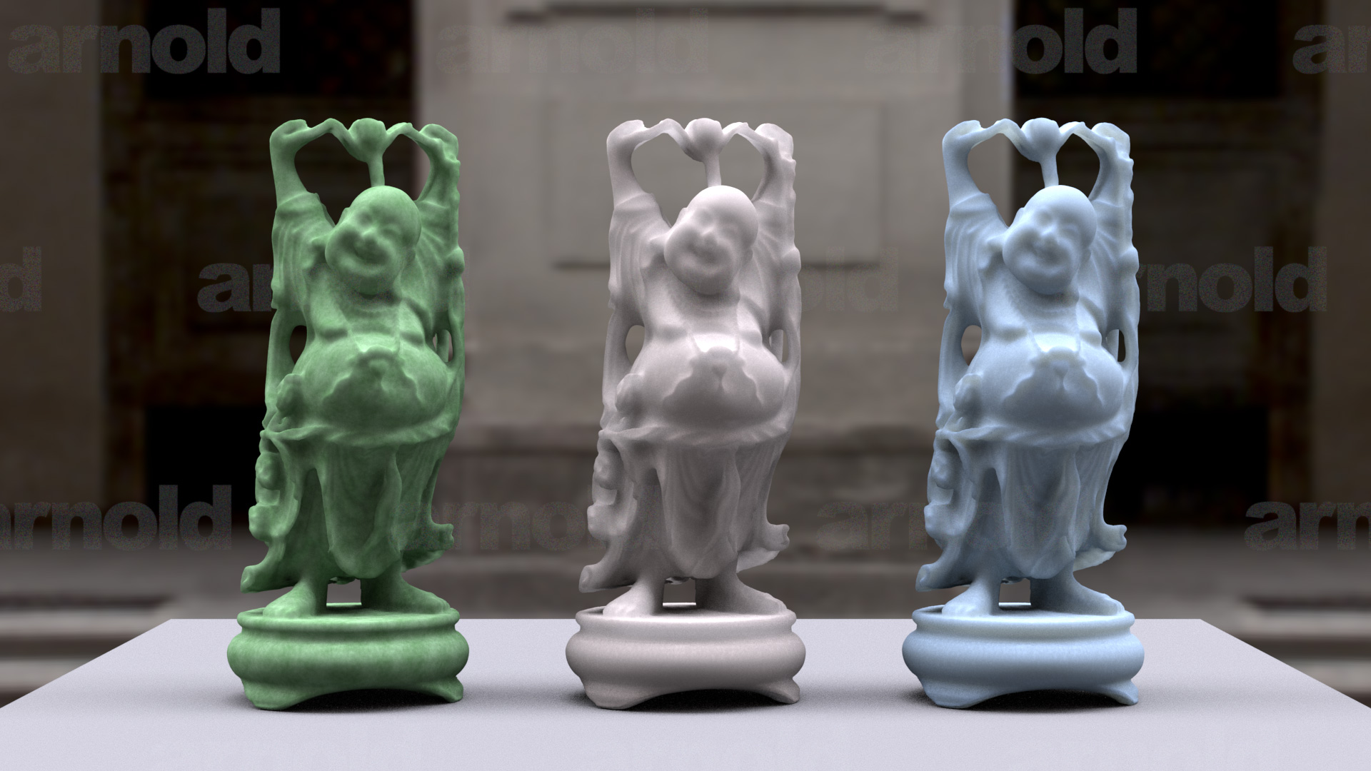
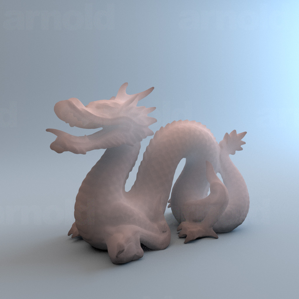
Results
References
- Jensen, Henrik Wann, et al. “A practical model for subsurface light transport.” SIGGRAPH 2001.
- Donner, Craig Steven. Towards realistic image synthesis of scattering materials. PhD Thesis, University California, San Diego, 2006.
- Habel, Ralf, Per H. Christensen, and Wojciech Jarosz. “Classical and Improved Diffusion Theory for Subsurface Scattering.” Technical Report, 2013.
- King, Alan, et al. “BSSRDF importance sampling.” SIGGRAPH Talks, 2013.
- Burley, Brent. “Extending the Disney BRDF to a BSDF with Integrated Subsurface Scattering.” SIGGRAPH Course Notes, 2015.
- Christensen, Per H., and Brent Burley. “Approximate reflectance profiles for efficient subsurface scattering.” Technical Report 15-04, Pixar, 2015.
comments powered by Disqus