Radial Basis Functions (RBFs) is one of the commonly used methods to interpolate multi-dimensional data. RBFs creates smooth and less oscillating interpolation than inverse distance weighting (IDW) does. It has many applications in Computer Graphics, such as surface reconstruction [3], animation blending [1], facial retargeting, color calibration [4], and etc. Despite of the variety of its applications, those applications all have a common theme called scattered data interpolation.

Scattered Data Interpolation

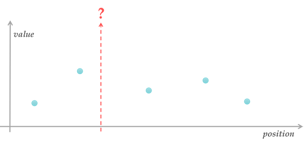
The problem of scattered data interpolation can be stated as:

given $n$ p-dimensional data points $\mathbf{x_1, x_2, …, x_n} \in \R^p$ with corresponding scalar values $f_1, f_2, …, f_n \in \R$,
compute a function $\tilde{f}({\bf x}): \R^p \to \R$ that smoothly interpolates the data points at other locations in $\R^p$ and exactly passes through $\mathbf{x_1, x_2},\ …,\ \mathbf{x_n}$

$$\tilde{f}(\mathbf{x_i}) = f_i,; for\ 1 \le i \le n$$

Those points have no particular structure, they are just scattered in p-dimensional space. In 1D, we could simply use piecewise linear interpolation. However, in order to extend this concept to 2D, we need to tessellate the spatial domain of the given data into triangular mesh and to use barycentric coordinates as blending weights. In 3D, we need to construct a tetrahedral mesh for interpolation instead.

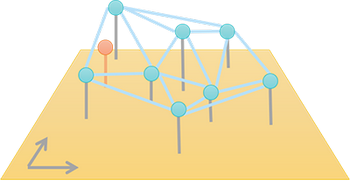
Fig. 1. Interpolation with triangular mesh on 2D surface.

This shows that the interpolation results are dependent on the intermediate structure (e.g. triangular or tetrahedral mesh). Additionally, as dimension gets higher, the interpolation cost of such generalization becomes much higher. Therefore, we want to seek an approach to interpolate data points without explicit tessellation in spatial domain.

Inverse Distance Weighting & Shepard’s Method

In multi-dimensional space, when we get closer to certain data point $\mathbf{x}_i$, we expect the value is also getting closer to $f_i$. Intuitively, we might assign blending weight according to the reciprocal of distance between a query position $\bf x$ and the data point $\mathbf{x}_i$:

$$\tilde{f}({\bf x}) = \sum_{i=1}^n{\frac{w_i({\bf x})}{\sum_j w_j({\bf x})} f_i},\quad w_i({\bf x}) = \frac{1}{\Vert{\bf x - x_i}\Vert} $$

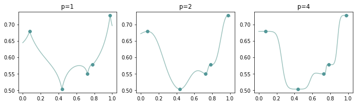
Unfortunately, this naive interpolation is not smooth around the data points. To make the interpolation smoother, we could raise blending weights to the power of $p: w_i({\bf x}) = {\Vert{\bf x - x_i}\Vert}^{-p},, p>0$. This inverse distance weighting technique is called Shepard’s method [1].

Even though $\tilde{f}$ is smooth at the interpolated points when $p>1$, but it also produces flat spots around the data points because the first derivative of $\tilde{f}$ w.r.t. $\bf x$ approaches 0 at all data points [6, page 518]. These flat spots cause unnecessary oscillation of interpolation (see Figure 2). This makes us wonder how could we get a smooth and less oscillating interplant.

Shepard interpolation with different values of p — Fig. 2. Shepard's interpolation with different values of $p$.

Blending with Basis Functions

To generalize the idea of inverse distance weighting, we could use a univariate function $\Phi: [0, \infty] \rightarrow \R$ to describe weights related to distances. But due to the overlapping ranges of influences between data points, using those distance related weights alone could not make the composed function pass through all data points as shown as below.

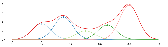
Summation of Gaussian basis functions — Fig. 3. Summing up Gaussian kernels alone fails to pass through all data points.

Thus we have to add extra scale factor $w_i$ to ensure the value at $x_i$ is $f_i$.

$$\tilde{f}({\bf x})=\sum_{i=1}^n{w_i \Phi(\Vert{\bf x-x_i}\Vert)},; \tilde{f}({\bf x_i})=f_i,; for; 1 \le i \le n$$

The kernel function $\Phi$ is called a radial function since it only depends on distances $\Vert {\bf x - x_i}\Vert$, so all locations on the hyper sphere have the same value. Let $\Phi_{i,j}=\Phi(\Vert{\bf x_i-x_j}\Vert)$, the linear system of equations is

$$\begin{bmatrix} \Phi_{1,1} & \Phi_{1,2} & \ldots & \Phi_{1,n} \\ \Phi_{2,1} & \Phi_{2,2} & \ldots & \Phi_{2,n} \\ \vdots & \vdots & \ddots \\ \Phi_{n,1} & \ldots & & \Phi_{n,n} \end{bmatrix} \begin{bmatrix}w_1 \\ w_2 \\ \vdots \\ w_n \end{bmatrix}=\begin{bmatrix} f_1 \\ f_2 \\ \vdots \\ f_n \end{bmatrix} \Rarr \mathbf{\Phi w = f}$$

For multi-dimensional ${\bf f}$, the matrix ${\bf \Phi}$ is the same, but the weights are solved for each dimension respectively.

$$\begin{bmatrix} \Phi_{1,1} & \Phi_{1,2} & \ldots & \Phi_{1,n} \\ \Phi_{2,1} & \Phi_{2,2} & \ldots & \Phi_{2,n} \\ \vdots & \vdots & \ddots \\ \Phi_{n,1} & \ldots & & \Phi_{n,n} \end{bmatrix} \begin{bmatrix} w_{1,1} & w_{1,2} \\ w_{2,1} & w_{2,2} \\ \vdots & \\ w_{n,1} & w_{n,2} \end{bmatrix} = \begin{bmatrix} f_{1,1} & f_{1,2} \\ f_{2,1} & f_{2,2} \\ \vdots \\ f_{n,1} & f_{n,2} \end{bmatrix}$$

To compute the interplant $\tilde{f}$, we have to choose a distance metric and a kernel function first. The common distance metric is Euclidean norm, while the selection of kernel is different to each specific application [1]. The figure below shows the influences of kernel selections for 1D interpolation:

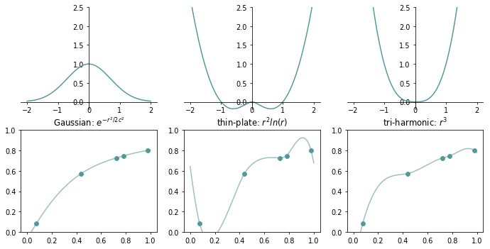
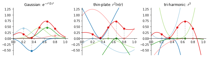
Fig. 4. Interpolation with various RBF kernels.

One counterintuitive point is that the some kernels are NOT inversely proportional to the distance at all, sometimes they even return zero at the data point! Take tri-harmonic for example, its value is in proportion to the distance between the query location and the data point. It works fine because we have extra weights $w_1, \dots, w_n$ to reconcile the differences (see Figure 5).

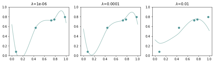
Fig. 5. RBF composition with various kernels: given data points shown in red, extra weights $w_i$ could reconcile the differences and make the interpolant pass through all the data points.

Now, our goal is to solve the weights $w_1, w_2, \ldots, w_n$. There are $n$ unknowns and $n$ equations. If there are no nearly the same rows in matrix ${\bf \Phi}$, the system should have a unique solution. Otherwise, the system would become ill-conditioned. To tackle this numerical problem, we add a regularizer $\mathbf{w}^{T}\mathbf{w}$ for the preference of diffuse weights to the objective function rather than solving ${\bf \Phi w = f}$ directly. While this also makes the function $\tilde{f}$ become an approximation instead of an interpolation of data points (i.e. $\tilde{f}$ no longer passes through the given data points as illustrated in Figure 6).

$$E({\bf w})=\Vert{\bf \Phi w - f}\Vert^2 + \lambda \Vert{\bf w}\Vert^2$$

In order to find the weights which minimize the objective function $E({\bf x})$, its derivative w.r.t. $\bf w$ should be zero:

$$\frac{\partial E}{\partial \bf w}=2 \mathbf{\Phi}^T({\bf \Phi w - f}) + 2\lambda {\bf w} = 0$$

$$({\bf \Phi^T \Phi} + \lambda \mathbf{I}) \mathbf{w} = \mathbf{\Phi}^T \mathbf{f}$$

$$\mathbf{w} = (\mathbf{\Phi}^T \mathbf{\Phi} + \lambda \mathbf{I})^{-1} \mathbf{\Phi}^T {\bf f}$$

As shown in Figure 6, when the regularization weight $\lambda$ is increasing, $\tilde{f}$ is getting less fitted to the data points. Sometimes our data might have outliers, regularization could help us avoid overfitting to the noise of data and improve the numerical stability of our system.

Thin-plate RBF with regularization — Fig. 6. Thin-plate RBF interpolation with regularization weights: $\lambda =$ 1e-6, 1e-4 and 1e-2.

Reproducing Polynomials

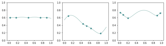
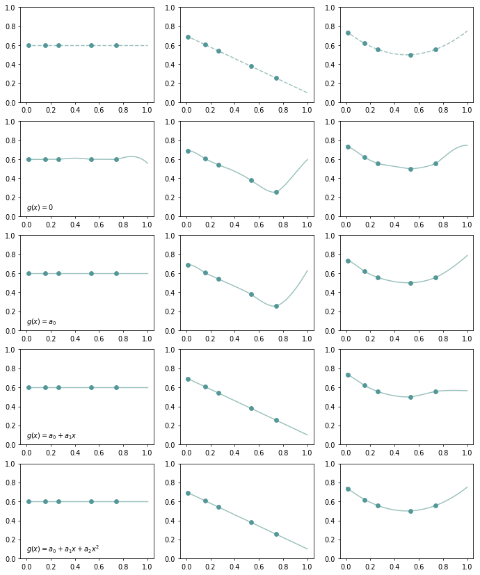
With radial basis functions, we could properly interpolate data at locations $\bf x_1, \ldots, x_n$. But that composed function $\tilde{f}$ may not be able to represent a polynomial function evaluated at other locations. Figure 7 shows how does the thin-plate kernel $r^2 \log{r}$ interpolate the data generated from a constant, linear and quadratic function:

Basis functions summation — Fig. 7. Thin-plate RBF interpolations from the samples of constant, linear and quadratic functions.

To make our interpolant able to represent polynomial function, we append monomials $\mathbf{g(x)=b(x)}^T \mathbf{c}$ to our interpolant. Let $\Pi^p_m$ be the set of polynomials with $p$ variables whose total degree is $m$. For instance, polynomials functions in $\Pi^2_2$ could be $c_1,\ c_1 + c_2 x + c_3 y,\ c_1 + c_2 x + c_3 y + c_4 x^2 + c_5 xy + c_6 y^2,; c_1, \dots, c_6 \in \R$.

Now, we have extra unknown coefficients $c_j$. There are more unknowns than the number of equations (underdetermined system), thus we need to add other constraints to get a unique solution of $w_i$ and $c_j$. Let $\bf P$ be the polynomial basis $\mathbf{b(x)}^T$ and $\bf c $ be the coefficients of the polynomial basis. Then the linear system becomes

$$\mathbf{\Phi w + P c = f}$$

and for ${\bf g(x)} \in \Pi^1_2, \bf{P}$ is in the form as

$$\mathbf{P}=\begin{bmatrix}1 & x_1 & x_1^2 \\ 1 & x_2 & x_2^2 \\ \vdots \\ 1 & x_n & x_n^2\end{bmatrix}$$

The additional relation we are looking for is that if the polynomial terms $\bf Pc$ exactly match the data points, we want the weights $w_i$ of radial basis functions all become zero. Suppose $\bf f$ could be exactly represented by the same polynomial basis with other coefficients $\bf d$

$$\mathbf{\Phi w} + \mathbf{Pc} = \mathbf{Pd}$$

and pre-multiply each term by $\mathbf{w}^T$

$$\mathbf{w}^T \mathbf{\Phi w} + \mathbf{w}^T \mathbf{Pc} = \mathbf{w}^T \mathbf{Pd}$$ $$\mathbf{w}^T \mathbf{\Phi w} = \mathbf{w}^T \mathbf{P(d-c)}=0$$

By requiring $\mathbf{w}^T \mathbf{P=0}$, then the left hand side $\mathbf{w}^T \mathbf{\Phi w}$ has to be zero, thus ${\bf w = 0}$. This also implies ${\bf Pc}$ is identical to $\bf Pd$ when $\bf w = 0$, the polynomial is exactly reproduced. Now the system with orthogonal constraint $\mathbf{w}^T \mathbf{P=0}$ is

$$\begin{bmatrix}\bf \Phi & \bf P \\ \mathbf{P}^T & \bm{0} \end{bmatrix} \begin{bmatrix}\bf{w} \\ \bf{c}\end{bmatrix} = \begin{bmatrix}\bf{f} \\ \bf{0}\end{bmatrix}$$

The following figure shows the capacities of polynomials with total degree 0, 1, 2. With extra polynomial terms, we could fit function with less oscillation.

Conclusion

Solving linear system takes $O(N^3)$, if there are too many data points (e.g. over several thousands), RBFs may not be a practical approach for interpolation. In this situation, we could use compact kernels (i.e. restrict the influence region of each data point) or solve the linear system iteratively [2].

I recently used RBFs for color calibration (matches color patches in ColorChecker) [4] and found it provides a more precise approximation than the method used in Far Cry3 [5, page 4](which uses a combination of two affine transformations and a polynomial regression in-between). We have also used RBFs to deform facial geometry with facial landmarks and got satisfactory results.

When dealing with data interpolation in high dimension, RBFs is a nice choice to generate smooth interpolation with low oscillation. Moreover, we could also add polynomial terms to increase the capacity of interplant and apply regularization to avoid data overfitting.

The python script that creates all figures in this post could be found here.

References

Ken Anjyo, J.P. Lewis, Frédéric Pighin. 2014. Scattered Data Interpolation for Computer Graphics. SIGGRAPH Course Notes.
Mario Botsch and Leif Kobbelt. 2005 Real-Time Shape Editing using Radial Basis Functions. Eurographics.
Daniel Cohen-Or, Chen Greif, Tao Ju, Niloy J. Mitra, Ariel Shamir, Olga Sorkine-Hornung, Hao (Richard) Zhang. 2015. A Sampler of Useful Computational Tools for Applied Geometry, Computer Graphics, and Image Processing. CRC Press.
Johannes Hanika. 2016. Colour manipulation with the colour checker lut module.
Stephen McAuley. 2012. Calibrating Lighting and Materials in Far Cry 3. SIGGRAPH Course Notes.
Donald Shepard. 1968. A two-dimensional interpolation function for irregularly-spaced data. Proceedings of the 1968 ACM National Conference. pp. 517–524.
Wilna du Toit. 2008. Radial Basis Function Interpolation. Master’s Thesis.