When I did homework assignments of the famous Deep Learning course CS231n from Stanford, I was so impressed by 100X↑ performance boost by using broadcasting mechanism in NumPy. However, broadcasting doesn’t always speed up computation, we should also take into account memory usage and memory access pattern [2], or we will get a slower execution instead. This post shows several experiments and my reasoning of why certain operation is performant or not.

Python List

The syntax of Python list is very similar to ndarray of NumPy, but their implementation of index operator is quite different. To avoid unnecessary memory copying, we have carefully to examine their differences.

Everything in Python is an object (a single integer object takes 28 bytes!) [4], the built-in function id() returns the identity of a given object, and is operator is used to compare object’s identity. While operator == is used to compare their representative values.

>>> i = 5
>>> sys.getsizeof(i)  # in bytes
28
>>> a = list(range(5))
>>> id(a)
1599991784136
>>> b = a
>>> b is a
True
>>> b[0] = 5
>>> b
[5, 1, 2, 3, 4]
>>> a
[5, 1, 2, 3, 4]
>>> c = [5, 1, 2, 3, 4]
>>> c is a  # They are different objects
False
>>> c == a  # But they have the same representative values
True

The expression b = a assigns the reference of a to b, then a and b points to the same memory afterword. If we want to perform element-wise copying, we could use b = a[:].

>>> a = list(range(5))
>>> b = a[:]
>>> b is a
False
>>> id(b), id(a)
(1599986754120, 1599991784136)

numpy.ndarray

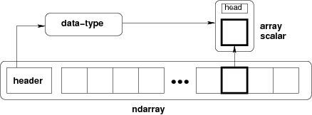
Python list is a heterogeneous data structure. To make it more efficient for massive numerical computation, NumPy provides a specialized multi-dimensional, homogeneous fixed-size array which contains block of memory, indexing scheme, and data descriptor [6].

>>> a = np.random.rand(5, 3)
>>> a.__array_interface__
{'data': (2294109792688, False), 
 'strides': None, 
 'descr': [('', '<f8')], 
 'typestr': '<f8', 
 'shape': (5, 3), 
 'version': 3}

>>> a.flags
  C_CONTIGUOUS : True
  F_CONTIGUOUS : False
  OWNDATA : True
  WRITEABLE : True
  ALIGNED : True
  WRITEBACKIFCOPY : False
  UPDATEIFCOPY : False

The address of internal memory block is stored at a.__array_interface__['data'][0]. When we write b = a[:], the slice syntax [:] for ndarray returns a view of internal data array, but fancy indexing such as a[a > 0] returns a new copy of array instead [1]. To see if they share the same memory block or not, we could check their base object. (The data ownership can be simply checked from the OWNDATA property of flagsobj.)

def get_base_array(a):
    """Get the ndarray base which owns memory block."""
    if isinstance(a.base, np.ndarray):
        return get_base_array(a.base)
    return a

def share_base(a, b):
    return get_base_array(a) is get_base_array(b)

a = np.random.rand(6, 4)
print('a, a[2:, 1:]       ->', share_base(a, a[2:, 1:]))    # True
print('a, a[a> 0]         ->', share_base(a, a[a > 0]))     # False
print('a, a.copy()        ->', share_base(a, a.copy()))     # False
print('a, a + 2           ->', share_base(a, a + 2))        # False

Here, we notice that a + 2 returns a new copy of array. If we don’t need extra copy, we had better use in-place operations like a += 2. By contrast, matrix transpose() and reshape() only changes the strides property, thus they have identical base array. Another thing should be noticed here is that even though both ravel() and flatten() have similar semantics, but ravel() returns a view if possible, while flatten always returns a new copied array [1].

print('a, a.transpose()   ->', share_base(a, a.transpose()))        # True
print('a, a.reshape(8, 3) ->', share_base(a, a.reshape(8, 3)))      # True
print('a, a.ravel()       ->', share_base(a, a.ravel()))            # True*
print('a, a.flatten()     ->', share_base(a, a.flatten()))          # False

If we want to check whether two array objects have overlapped memory or not, we could use numpy.shares_memory(). It helps us tell the difference between A[::2] and A[1::2].

Locality Matters

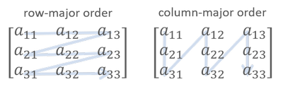
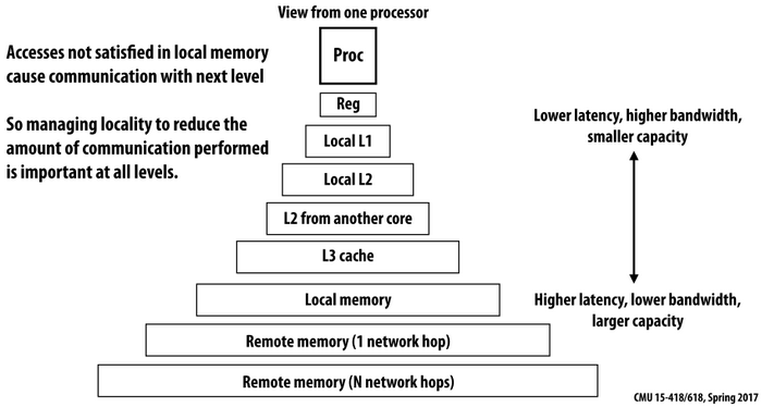
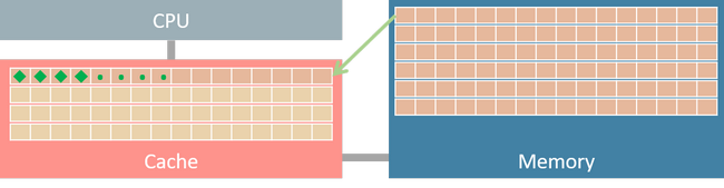
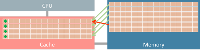
In NumPy, ndarray is stored in row-major order by default, which means a flatten memory is stored row-by-row. When frequently accessing elements of a massive array, memory access pattern would dramatically affect computation performance [2]. Figure 1 shows the memory hierarchy of a computer system. Data are transferred between memory and cache in blocks of fixed size (typically in 64 bytes) called cache line.

Suppose we have a float32 matrix X with 5,000 by 5,000 elements. Each float32 element takes 32 bits = 4 bytes, and its total storage size is 25,000,000 x 4 bytes = 100 MB.

If matrix X is stored in row-major order, then its strides is (20000, 4). It indicates that increasing row index by one strides 20,000 bytes in memory. Since the strides for column index is 4 bytes, we could get 64 / 4 = 16 consecutive elements in one data transaction (assume the size of a cache line is 64 bytes). If we iterative array elements in row-major order, after a data fetching requested for the first element, the next 15 elements are also in cache, thus the subsequent access of these 15 elements only takes few clock cycles.

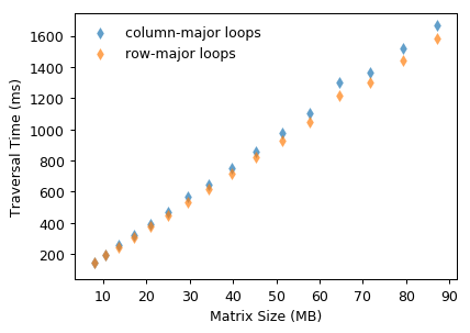
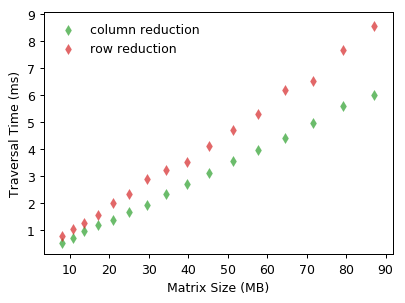
On the contrary, if we traverse the matrix in column-major order (varies the leftmost array index in inner loops), two adjacent access X[r, c], X[r+1, c] fetch two different cache lines. It fetches 16 elements from memory to cache, but it only uses one element of them and never touches the others before cache eviction. Such inefficient data utilization reflects on higher traversal time shown in Fig. 4.

Vectorization

As mentioned before, everything in Pythion is an object. A Python integer is more than just an integer, it also contains other information that wraps the raw data. When traversing a list of integers, it takes few times of indirect access before retrieving the actual data. Moreover, there are some other costs of type checking and function dispatching for dynamic typing process [4].

This would be very inefficient when the list size gets larger and larger. Because that list only has homogeneous elements, we don’t want to pay extra costs for the support of heterogeneous elements. Instead, we tend to use NumPy ndarray and element-wise operations to turn Python explicit loops into implicit loops in low-level implementation like CPython. Such element-wise operations that operate on entire arrays is called a vectorized operations.

# Explicit loops in row-major order.
total = 0
for i in range(rows):
    for j in range(cols):
        total += A[i, j]

# Implicit loops in a vectorized operator.
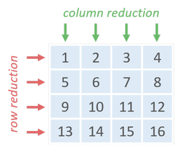
total = np.sum(np.sum(A, axis=1))  # Row reduction first.
total = np.sum(np.sum(A, axis=0))  # Column reduction first.

With vectorization, the traversal time decreases significantly by using row or column reduction. Vectorized array operations outperform explicit Python for-loops nearly 200X when the matrix size is around 90 MB.

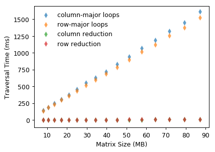
Likewise, memory access order also affects the performance of row or column reduction. But one thing should be noticed is that summing elements along rows (i.e. column reduction) is faster than the other that accumulates along columns.

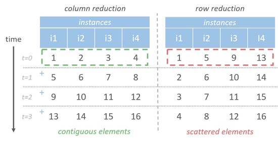
Vectorized array operations are parallelly executed possibly with SIMD or multi-threading [9] mechanism. If we fetch data row-by-row, we could easily accumulate elements of each column in parallel. Let there be 4 parallelly executing instances, at each time they could execute one identical instruction on different data. In column reduction order, each instance operates on contiguous elements which could be fetched in one data transaction. While the elements required for row reduction each time (ex. [1, 5, 9, 13]) are scattered somewhere, it has to take more clock cycles to fetch them all.

Using Matrix Multiplication for Reduction

Now, let’s go one step further. Row reduction could be formulated as a matrix multiplies a column vector with ones, and column reduction is equal to a row vector of ones multiplies a matrix (or a transpose matrix multiplies a column vector of ones).

np.sum(np.sum(A, axis=1))           # Row reduction.
np.sum(A.dot(np.ones(A.shape[1]))   # Row reduction by using dot product.

np.sum(np.sum(A, axis=0))           # Column reduction first.
np.sum(A.T.dot(np.ones(A.shape[0])) # Column reduction by using dot product.

np.sum(A)   # Matrix reduction

Surprisingly, this is the fastest way for matrix reduction! It takes 6 ms to reduce a float64 matrix of 5,000 by 5,000 elements with i7-9700K and 32 GB of RAM.

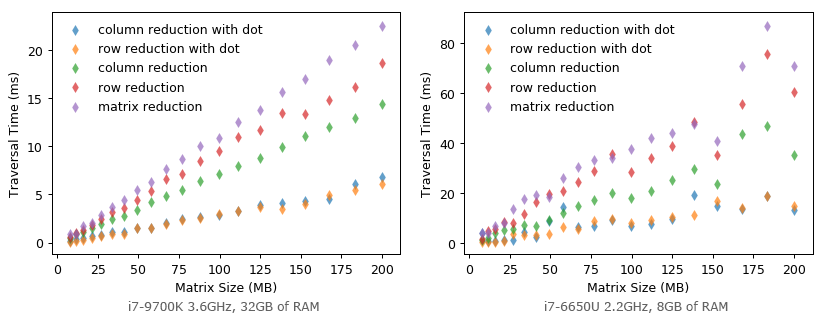
Could it be even faster when we halve the size of matrix element to float32 (double the elements that can be fetched in one cache line transaction)? Unfortunately, it becomes much SLOWER! It seems that matrix multiplication is highly optimized for float64 specifically?

I’m curious about such results. I’m not sure if this is a special case on my machine or not. For those people who are also curious about it, here is the source code. If you have got different results, please drop me a note or leave comments. My testing environment is Python 3.7.2 64-bit with NumPy 1.16.2 on Windows 10.

Broadcasting

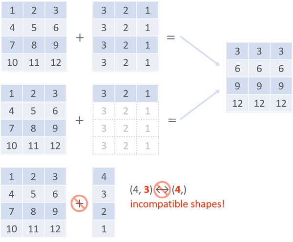
Basic operations on ndarrays are element-wise. Before applying operations on two arrays, we have to stretch their shapes to make them match. To avoid such needless copies of data, there is a powerful mechanism called broadcasting. It performs arithmetic operations on compatible ndarrays with different shapes by means of vectorizing array operations.

When operating on two arrays, the compatibility check of broadcasting starts from the trailing dimensions to the heading ones. Two dimensions are compatible if they are equal or one of them is 1.

In general, broadcasting improves computing performance due to array vectorization (i.e. the iterations occurs in C instead of Python) and the avoidance of redundant data copying. However, if broadcasting uses more memory than explicit loops do, it might become slower instead.

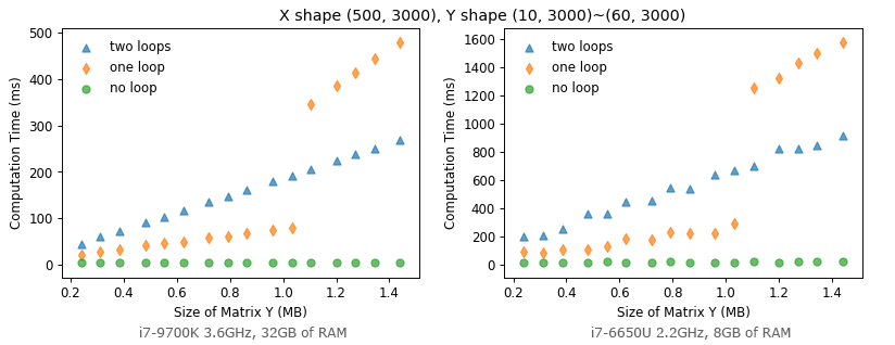
Let each data sample be in N dimensions, and two data set X, Y be with M_X and M_Y samples respectively. Suppose we want to compute the Euclidean distance (L2 norm) between all sample pairs in X, Y. If we format the dataset in matrix form X[M_X, N], and Y[M_Y, N], here are three implementations:

1. norm_two_loop: two explicit loops
2. norm_one_loop: broadcasting in one loop
3. norm_no_loop: broadcasting with no loop

def norm_two_loop(X, Y):
    dists = np.empty((X.shape[0], Y.shape[0]))
    for i in range(X.shape[0]):
        for j in range(Y.shape[0]):
            # The memory usagee is two (N,) vectors.
            dists[i, j] = np.sqrt(np.sum((X[i] - Y[j]) ** 2))
    return dists

def norm_one_loop(X, Y):
    dists = np.empty((X.shape[0], Y.shape[0]))
    for i in range(X.shape[0]):
        # The memory usage here is (N,) plus (MY, N) from Y.
        dists[i, :] = np.sqrt(np.sum((X[i] - Y) ** 2, axis=1))
    return dists

def norm_no_loop(X, Y):
    X_sqr = np.sum(X ** 2, axis=1)  # X_sqr.shape = (MX,)
    Y_sqr = np.sum(Y ** 2, axis=1)  # Y_sqr.shape = (MY,)
    # X.dot(Y.T) takes two 1D vectors in its implicit loop on at a time.
    # The shapes of entire broadcasting process are: (MX, 1) - (MX, MY) + (MY,)
    # => (MX, MY) + (MY)
    dists = np.sqrt(X_sqr[:, np.newaxis] - 2.0 * X.dot(Y.T) + Y_sqr)
    return dists

As we suggested before, computing performance is related to memory usage and memory access pattern. For X[500, 3000] and Y[10~60, 3000], norm_one_loop gets slower than norm_two_loop when its memory usage exceeds about 1 MB. Such performance drop might be due to the required data can’t fit in the cache, so it has to retrieve those data from external memory which is much slower in an order of magnitude (10X↑ slower).

CacheFun is a fantastic web page which demonstrates the speed differences between L1$, L2$ and main memory. Don’t miss it!!

Then, what if we transpose Y into a tall matrix whose shape is (30, 1000) ~ (180, 1000)? (This implies norm_two_loop takes more iterations in its inner loops.)

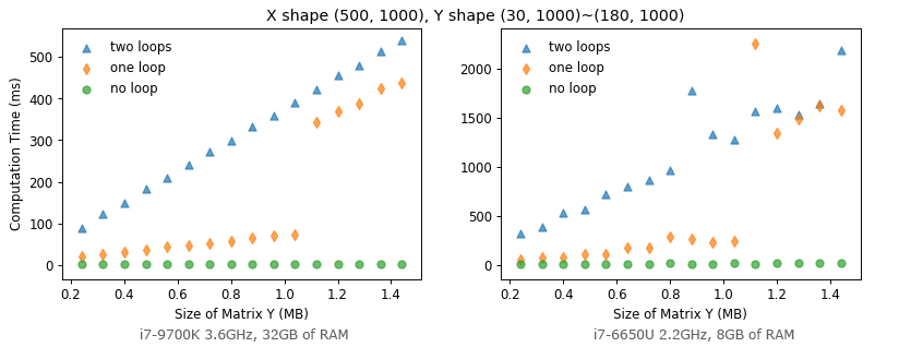
Figure 13 shows norm_one_loop still gets a performance drop when the memory usage exceeds about 1MB, but it’s mostly faster than norm_two_loop now. This confirms that looping in Python takes a significant amount time. Whenever possible, we should avoid explicit iterating over arrays in Python as much as possible. Broadcasting is performant in general, but we need to be aware of its memory usage to avoid a performance drop.

Conclusion

To wrap it up, the general performance tips of NumPy ndarrays are:

1. Avoid unnecessarily array copy, use views and in-place operations whenever possible.
2. Beware of memory access patterns and cache effects.
3. Vectorizing for-loops along with masks and indices arrays.
4. Use broadcasting on arrays as small as possible.

About other optimization techniques, please refer to these wonderful articles [3], [5], [7] and [8]. This is what I have learned so far, hope you will like to use NumPy for numerical computing as I do. :)

ps. The python script that creates all figures in this post could be found here, and here is the Jupyter notebooks of my testing results with i7-9700K and i7-6650U.

References

1. Alex Chabot-Leclerc. 2018. Intro to Numerical Computing with NumPy [slides], SciPy Conference.
2. Scott Meyers. 2013. CPU Caches and Why You Care [slides], code::dive Conference.
3. Cyrille Rossant. 2018. Chapter 4, Profiling and Optimization, IPython Cookbook 2/e.
4. Jake VanderPlas. 2016. Understanding Data Types in Python, Python Data Science Handbook.
5. Gaël Varoquaux, Optimizing Code, SciPy lecture notes.
6. Pauli Virtanen. Advanced NumPy, SciPy lecture notes.
7. Stéfan van der Walt, S. Chris Colbert, Gael Varoquaux. 2011. The NumPy Array: A Structure for Efficient Numerical Computation. Computing in Science and Engineering.
8. How to optimize for speed, scikit-learn documentation.
9. Parallel Programming with Numpy and SciPy.