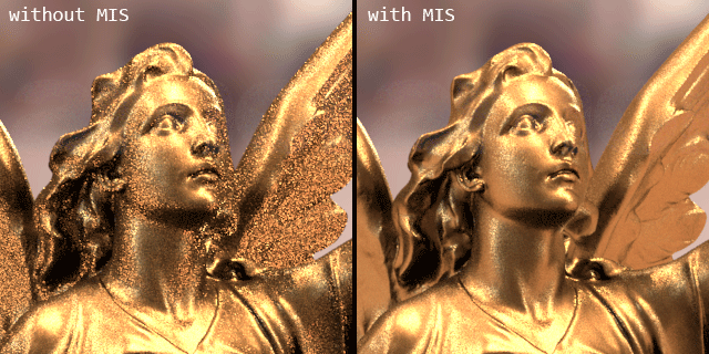
Monte Carlo path tracing has a slow convergence rate close to \(O(1/\sqrt n)\), it needs to quadruple the number of samples to halve the error. Many mainstream production renderers have deployed multiple importance sampling (MIS) technique to reduce the variance of sampling result (i.e. the noise in image). If we want to make our custom material shader efficiently executed along with the entire render scene in Arnold, we shall definitely consider exploiting the power of MIS.
What is Multiple Importance Sampling (MIS)?
Suppose we want to solve the direct illumination equation:
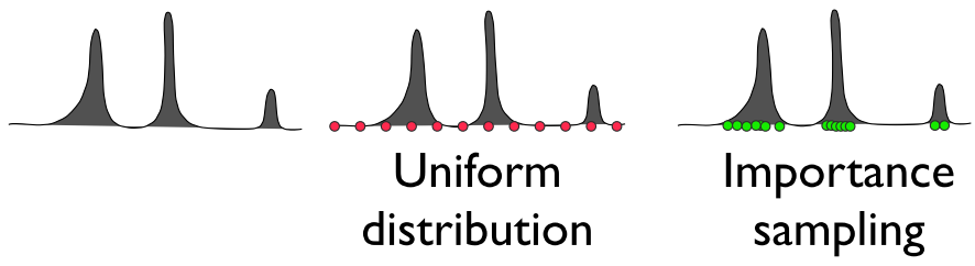
Monte Carlo sampling uses random samples to compute this integral numerically. The idea of importance sampling is trying to generate the random samples proportional to some probability density function (PDF) which has similar shape of the integrand.
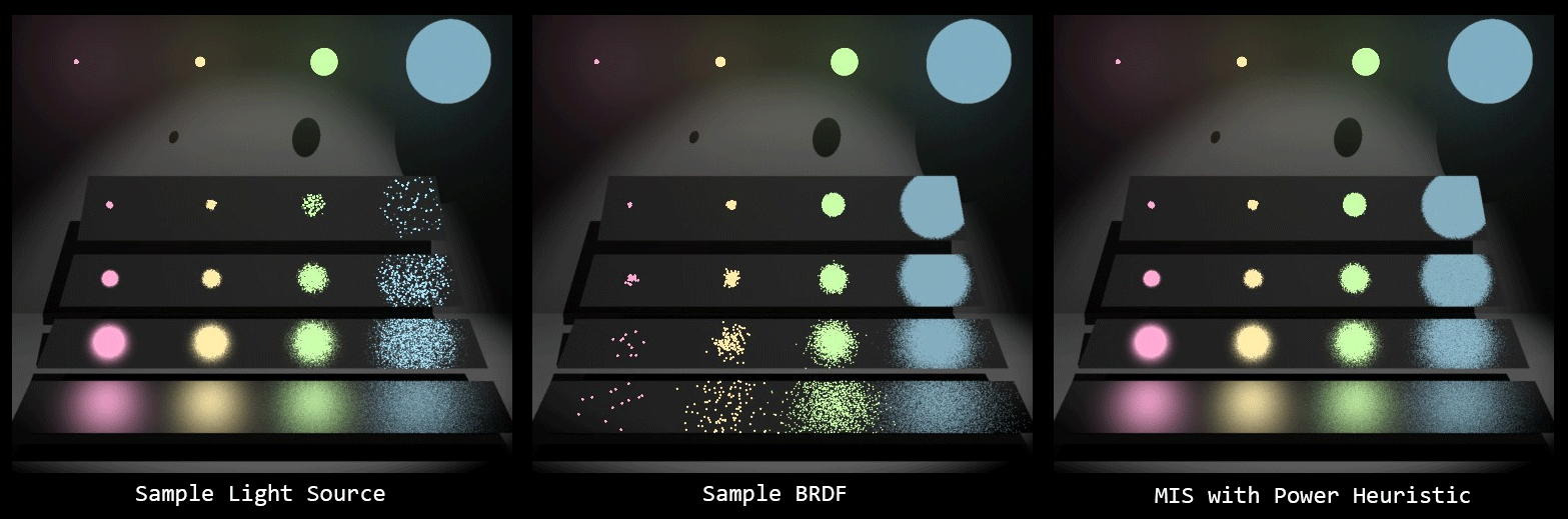
In other words, the ideal PDF for the integrand of direct illumination equation would be proportional to the product of incoming radiance \(L_i(x,\vec{\omega_i})\) and BRDF \(f_r(x,\vec{\omega_o}, \vec{\omega_i})\). However, the product of these terms are too complicated to compute its PDF, but we might be able to find a suitable PDF for some of those terms individually. What we hope is to find a way to sample each term respectively and properly combine those samples to get a result with lower variance. This turns to the technique named Multiple Importance Sampling (MIS) demonstrated by Veach and Guibas [1] in 1995:
With MIS, we use following formula to compute the result:
Where \(n_k\) is the number of samples taken from certain PDF \(p_k\). The weighting functions \(w_k\) takes all the different ways that a sample could have been generated, and \(w_k\) could be computed by power heuristic: $$w_k(x)=\frac{(n_s p_s(x))^\beta}{\sum_i{(n_i p_i(x))^\beta}}$$
The MIS API in Arnold
At each shading point, we want to compute the direct illumination and indirect illumination. In order to utilize MIS API in Arnold, we have to provide three functions:
- AtBRDFEvalPdfFunc
- AtBRDFEvalSampleFunc
- AtBRDFEvalBrdfFunc
For getting better understanding of the task of these functions. Recall that our goal is to use MIS to combine the samples generated from both PDFs of lights and BRDF. Let BRDF as \(f(X)\) and lighting function as \(g(Y)\) in equation (1), then the unknown entities to Arnold are:
- \(\textcolor{#FF3399}{p_f}\) (AtBRDFEvalPdfFunc): the PDF of BRDF
- \(\textcolor{#009933}{X_i}\) (AtBRDFEvalSampleFunc): the sample direction generated according to \(\textcolor{#FF3399}{p_f}\)
- \(\textcolor{#0099FF}{f}\) (AtBRDFEvalBrdfFunc): the BRDF evaulated with sampled incoming direction and fixed outgoing direction (i.e. -sg->Rd)
With these information, \(w_f(X_i)\) and \(w_g(Y_j)\) can be computed with power heuristic:
Now suppose we want to use GGX for glossy component, the shading structure would like this:
GgxBrdf ggx_brdf;
GgxBrdfInit(&ggx_brdf, sg);

auto directGlossy = AI_RGB_BLACK;

AiLightsPrepare(sg);
while (AiLightsGetSample(sg)) {
  if (AiLightGetAffectSpecular(sg->Lp)) {
    directGlossy += AiEvaluateLightSample(sg, &ggx_brdf,
      ggxEvalSample, ggxEvalBrdf, ggxEvalPdf);
  }
}

auto indirectGlossy = sg->Rr > 0
  ? AI_RGB_BLACK
  : AiBRDFIntegrate(sg, &ggx_brdf,
      ggxEvalSample, ggxEvalBrdf, ggxEvalPdf, AI_RAY_GLOSSY);
BRDF Evaluation
The content of ggxEvalBrdf is the formula of microfacet BRDF:
$$f_r(i,o,n)=\frac{F(i, h_r)G(i, o, h_r)D(h_r)}{4|i⋅n||o⋅n|}$$
- \(i, o\) are the incoming and outgoing direction
- \(h_r\) is the normalized half vector
- \(n\) is the macro-surface normal
- \(F\) is Fresnel term, \(G\) is masking/shadowing term and \(D\) is the microfacet normal distribution
Please refer to the paper of Walter et al. [2] for more details.
Evaluate the PDF for direction sampling
The job of ggxEvalPdf is to evaluate the PDF for given direction and it must match the density of samples generated by ggxEvalSample. The strategy suggested by Walter et al. [2] is to sample the microfacet normal \(m\) according to \(p_m(m)=D(m)\vert m\cdot n \vert\), and then transform the PDF from microfacet to macro-surface:
$$p_o(o)=p_m(m)\left|\frac{\partial\omega_h}{\partial\omega_o}\right|=\frac{D(m)|m⋅n|}{4|i⋅m|}$$
float ggxEvalPdf(const void *brdfData, const AtVector *indir)
{
    // V = -sg->Rd, Nf = sg->Nf
    auto M = AiV3Normalize(V + *indir);
    auto IdotM = ABS(AiV3Dot(V, M));
    auto MdotN = ABS(AiV3Dot(M, Nf));
    // We pass Nf to D(), since it needs to compute thetaM which is the angle
    // between microfacet normal M and macro-surface normal N.
    return D(M, Nf) * MdotN * 0.25f / IdotM;
}
Create the sample direction from PDF
In ggxEvalSample, the direction is sampled with the cosine weighted microfacet normal distribution:
$$p_m (m)=D(m)|m⋅n|\text{, where }D(m)=\frac{\alpha_g^2}{\pi\cos^4{\theta_m}(\alpha_g^2+\tan^2{\theta_m})^2}$$
With the distribution transformation from \(\omega_m\) to \(\theta_m, \phi_m\):
$$p_m(\theta_m, \phi_m)=\sin{\theta_m}\ p_m(m)$$
We can compute the marginal probability of \(p_m(\theta_m)\) and conditional probability \(p_m(\phi_m\vert\theta_m)\)
$$p_m(\theta_m)=\int_0^{2\pi}{D(m)\cos{\theta_m} \sin{\theta_m}\ d\phi_m} = \frac{2\alpha_g^2\sin\theta_m}{\cos^3{\theta_m}(\alpha_g^2+\tan^2{\theta_m})^2}$$
$$p_m(\phi_m\vert\theta_m) = \frac{p_m(\theta_m, \phi_m)}{p_m(\theta_m)} = \frac{1}{2\pi}$$
Then, we compute the corresponding CDFs and their inverse functions to get \(\theta_m, \phi_m\) from two canonial random variable \(\xi_1, \xi_2 \in [0, 1)\)
$$P_m(\phi_m|\theta_m) = \int_0^{\phi_m} \frac{1}{2\pi} d\phi’ = \frac{\phi_m}{2\pi}, \kern{1em} \phi_m = 2\pi \xi_2$$
Finally, we generate a sample direction with spherical coordinate \(\theta_m, \phi_m\) and transform the vector from local frame of shading point U, V, Nf(face-forward shading normal) into world space:
AtVector ggxEvalSample(const void *brdfData, float rx, float ry)
{
    // Sample microfacet normal.
    auto thetaM = atanf(roughness * sqrtf(rx / (1.0f - rx)));
    auto phiM = AI_PITIMES2 * ry;

    AtVector M;
    M.z = cosf(thetaM);
    float r = sqrtf(1.0f - SQR(M.z));
    M.x = r * cosf(phiM);
    M.y = r * sinf(phiM);

    // Transform the M from local frame to world space.
    // The U, V can be retrieved from AiBuildLocalFramePolar with sg->Nf.
    AiV3RotateToFrame(M, U, V, Nf);

    // Compute reflected direction according to view direction and normal vector.
    // V = -sg->Rd
    return 2.0f * ABS(AiV3Dot(V, M)) * M - V;
}
Results
In comparison to aiStandard, GGX has stronger tails than Beckmann which is used in aiStandard.
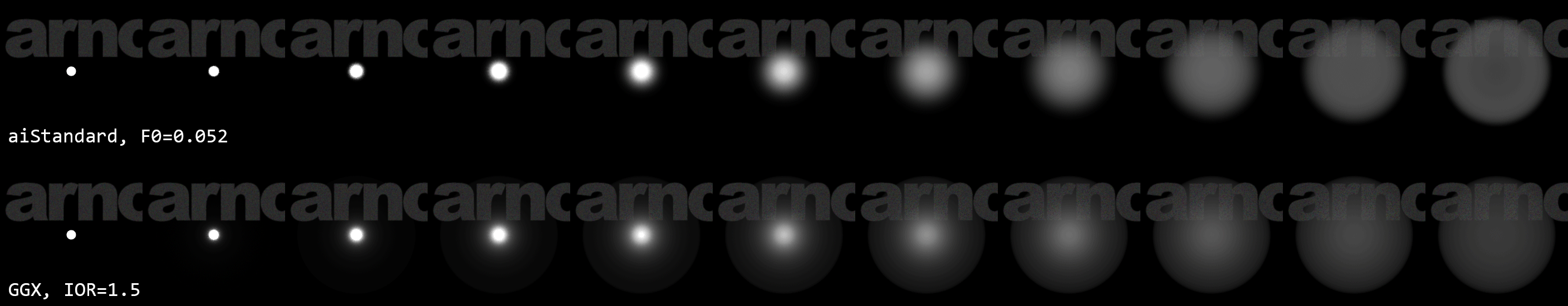
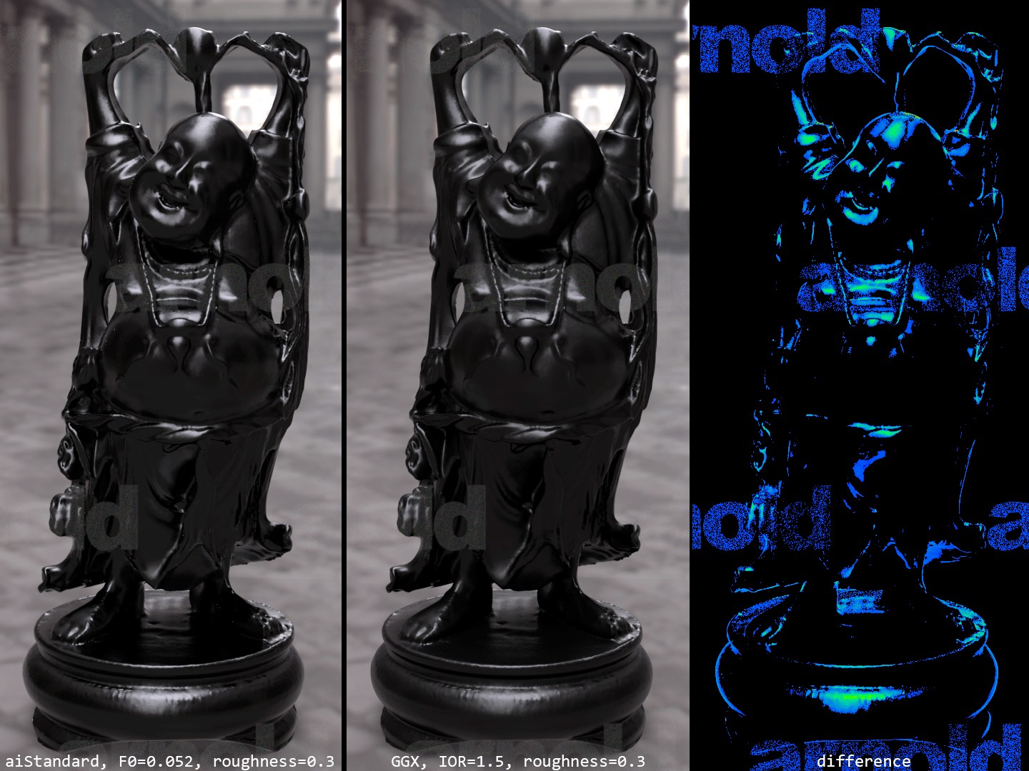](https://shihchinw.github.io/images/rlShaders/rlGgx_buddha_cmp.jpg)
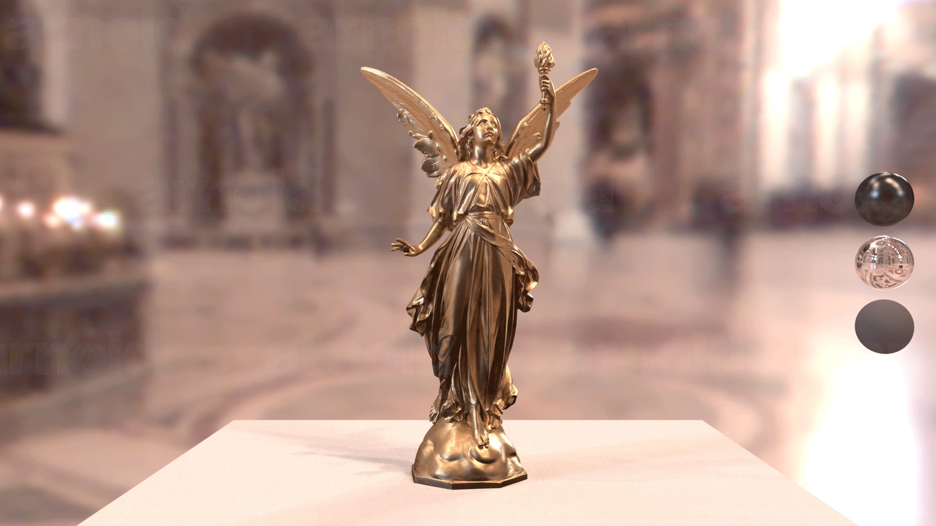
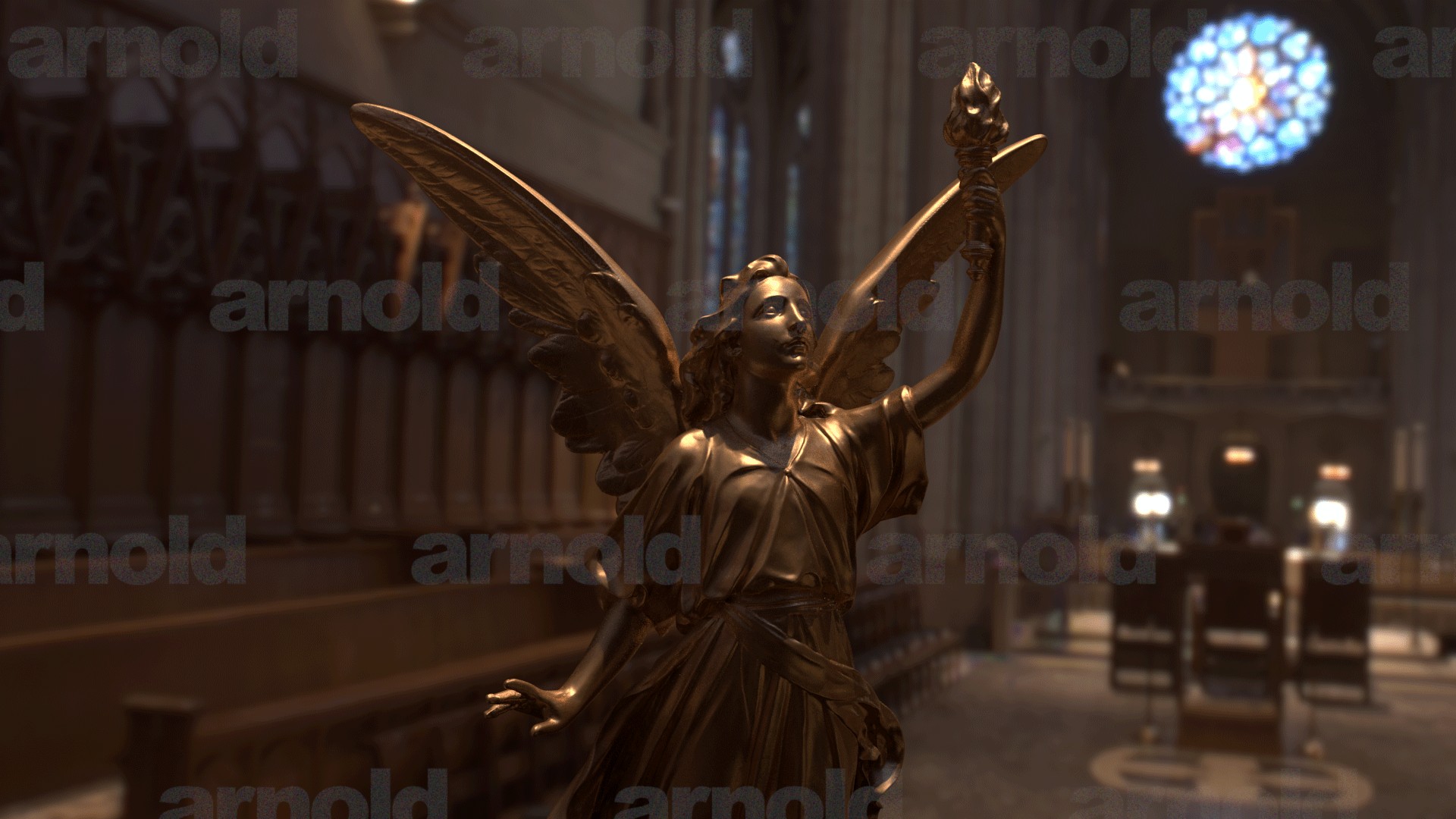
The results of the custom BRDF composed of GGX for glossy and Oren Nayar for diffuse.
References
- Veach, Eric, and Leonidas J. Guibas. "Optimally combining sampling techniques for Monte Carlo rendering." SIGGRAPH, 1995.
- Walter, Bruce, et al. "Microfacet models for refraction through rough surfaces." EGSR'07.
- Colbert, Mark, Simon Premoze, and Guillaume François. “Importance sampling for production rendering.” SIGGRAPH 2010 Course Notes.
- Pharr, Matt, and Greg Humphreys. Physically based rendering: From theory to implementation 2/e. Morgan Kaufmann. 2010.
comments powered by Disqus