The standard approach proposed by Walter et al. [1] for importance sampling of GGX BRDF is to use the PDF proportional to distribution of microfacet normal $D(\omega)$. However, $D(\omega)$ is not view-dependent, thus it would waste lots of samples when the incoming direction is near grazing angles. In addition, the small value of $D(\omega)\vert m\cdot n\vert$ at grazing angle would make the sample value as high as hundreds to millions in some situations and cause fireflies in render results.

In order to tackle these problems, Heitz and d’Eon [3] proposed a new method by sampling from the distribution of visible normals. Due to the consideration of view direction, their approach can significantly reduce the amount of wasted samples and make the sample weight in proper range to avoid the fireflies.

Revisit the Distribution of Normals $D(\omega)$

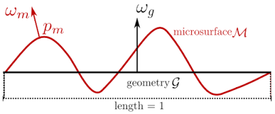
Suppose the area of macro surface is $1m^2$ and its normal is $\omega_g$. The normal of each microfacet point $p_m$ on the micro-surface $\mathcal{M}$ is $\omega_m(p_m)$ and the distribution of normals is:

$$D(\omega) = \int_\mathcal{M}{\delta_\omega (\omega_m(p_m)) dp_m}$$

The unit stated in Heitz [2] is $\frac{m^2}{sr}$ instead of $\frac{1}{sr}$, it’s different from the one stated in Walter et al. [1]

$D(\omega)$ describes the area of points $\mathcal{M}^{\prime} \subset \mathcal{M}$ whose normals lie in the given solid angle $\omega$. Additionaly, it relates the integral from microsurface space to the space the normals which is the unit sphere $\omega$:

$$microsurface\ area = \int_\mathcal{M}{dp_m} = \int_\Omega{D(\omega_m)d\omega_m}$$

and the projected area along the geometry normal $\omega_g$ is:

$$\int_\Omega{(\omega_m\cdot\omega_g) D(\omega_m )d\omega_m} = \int_\mathcal{M}{(\omega_m (p_m)\cdot\omega_g )dp_m}=1$$

The Distribution of Visible Normals $D_{\omega_o}(\omega)$

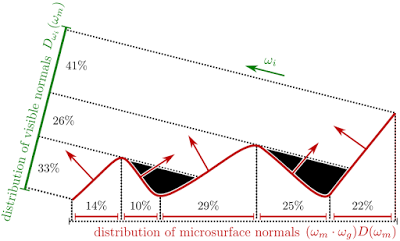
When we consider the projected area along the outgoing direction $\omega_o$, we have to add a masking function $\color{#009933}{G_1(\omega_o, \omega_m)}$ to exclude the occlusion part (i.e. the black parts in the figure above):

$$\int_\omega{\textcolor{#009933}{G_1(\omega_o, \omega_m)}\langle\omega_o, \omega_m\rangle D(\omega_m)d\omega_m}=\textcolor{#0099FF}{\cos{\theta_o}}$$

With these information, the outgoing radiance from the microsurface can be formulated as:

where the distribution of visible normals is $\textcolor{#FF3399}{D_{\omega_o}(\omega_m)} = \frac{1}{\cos{\theta_o}}G_1(\omega_o,\omega_m)\langle\omega_o, \omega_m\rangle D(\omega_m)$.

Importance Sampling of $D_{\omega_o}(\omega)$

For the anisotropic case, the $D(\omega_m)$ should be replaced with $D(\omega_m,\alpha_x,\alpha_y)$ and the distribution of visible normals becomes:

$$D_{\omega_o}(\omega_m,\alpha_x,\alpha_y) = \frac{1}{\cos{\theta_o}} G_1(\omega_o,\omega_m)\langle \omega_o, \omega_m \rangle D(\omega_m,\alpha_x,\alpha_y)$$

Since it’s not easy to perform importance sampling with $D_{\omega_o}(\omega_m,\alpha_x,\alpha_y)$ directly, Heitz and d’Eon [3] proposed a novel technique based on Heitz’s discovery [2] of stretch invariance property in slope space to accomplish the task.

Normal Vector in Slope Space

Suppose the microsurface is a heightfield, given a normal $\omega_m(x_m, y_m,z_m)$, its coordinate in slope space can be defined as:

and the distribution of slopes $P^{22}(\tilde{m})$ is necessarily normalized (all the possibilities must sum to 1):

Recall that $\int_\omega{(\omega_m\cdot\omega_g)D(\omega_m)d\omega_m} = 1$, we get the following relationship:

Likewise, the relationship involved with masking is (cf. Heitz [2] p.82):

where $P_{\omega_i}^{22}(\tilde{m})$ is the distribution of visible slopes, and it shows that if we sample the slopes from $P_{\omega_i}^{22}(\tilde{m})$ and transform them to normal $\omega_m$, the resulting PDF is $D_{\omega_i}(\omega_m)$.

Stretch Invariance

Suppose the distribution of slopes $P^{22}$ depends on the roughness $\alpha_x,\alpha_y$, Heitz calls $P^{22}$ is stretch invariant if changing its roughness would only stretch the distribution but keep its shape identical:

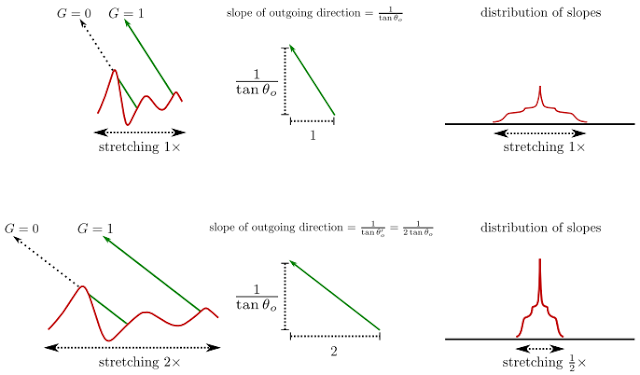
In 1D case, stretch x-axis by a factor of 2 would compress the distribution by 2 and also notice that the height of distribution has been scaled by 2. Suppose the distribution is $D(x, \alpha)$, the stretch invariance can be described as $D(x, \alpha) = \frac{1}{\lambda}D(\frac{x}{\lambda},\frac{\alpha}{\lambda})$.

Extend this relationship to 2D, we get:

In Heitz and d’Eon [3], they showed that the distribution of visible slopes also has the following relationship:

With stretch invariance property, any anisotropic distribution can be stretched into an isotropic one whose masking probability $G$ is the same. Then the samples can be generated with the help of the stretched isotropic distribution in following steps:

1. Apply stretch invariant property to make $P_{\omega_i}^{22}$ isotropic
2. Sample the slope coordinate $x_{\tilde{m}}$ according to the marginal PDF $P_{\omega_i}^{2-}(x_{\tilde{m}},\textcolor{#FF3399}{1,1})$
3. Sample $y_{\tilde{m}}$ with given $x_{\tilde{m}}$ and conditional PDF $P_{\omega_i}^{2|2}(y_{\tilde{m}}|x_{\tilde{m}},\textcolor{#FF3399}{1,1})$
4. Rotate along the z axis by $\phi$ in canonical frame
5. Inversely stretch the slope coordinate $(x_m, y_m)$
6. Compute normal from slope coordinate $\omega_m = \frac{(-x_m, -y_m, 1)}{\sqrt{x_m^2 + y_m^2 + 1}}$

The implementation details can be found in the supplemental document of the Heitz and d’Eon [3].

Experimental Results

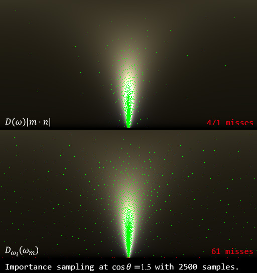
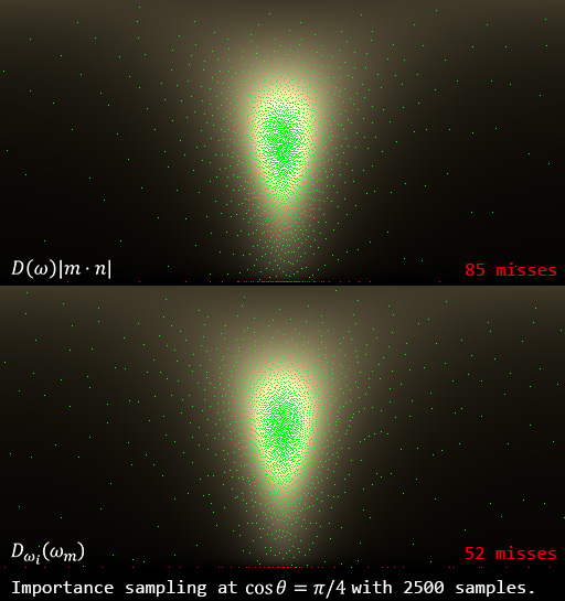
When $\cos{\theta_o}=1.5 (\theta_o\approx 85.94^\circ)$, the new method saves 310 wasted samples! The remaining 61 back-facing samples are about $1\sim3\degree$ below the macrosurface. However, the mysterious situation happens at $\cos{\theta_o}=\pi/4$. In current implementation, there still are 52 invalid samples whose maximum $\theta_i$ is about $3\pi/4$!! From the debugging traces, I found all those invalid samples come with a random number rx that is near to 0 or 1. To my best guess, this weird result may be caused by numerical errors and needs further investigation.

As usual, the implementation can be found on my github.

References

1. Walter, Bruce, et al. “Microfacet models for refraction through rough surfaces.” EGSR'07.
2. Heitz, Eric. “Understanding the Masking-Shadowing Function in Microfacet-Based BRDFs.” JCGT'14. [slides]
3. Heitz, Eric, and Eugene d’Eon. “Importance Sampling Microfacet‐Based BSDFs using the Distribution of Visible Normals.” EGSR'14. [source code][slides]